Math rabbit hole: Decaying lights
Here’s a fun problem that I came up with a while ago.
Suppose you have $n$ lightbulbs. All of them are initially on. On every second, each lightbulb independently has probability $p$ of turning off permanently. What is the expected amount of time you have to wait for all light bulbs to die? \(\newcommand{ev}[1]{\mathbb{E}\left[#1\right]} \newcommand{evt}[1]{\ev{T_{p}(#1)}} \newcommand{binom}[2]{ {#1 \choose #2} } \newcommand{bigo}[1]{\mathrm{O}\!\left( #1 \right) } \newcommand{prob}[1]{\mathbb{P}\!\left( #1 \right) }\)
Let’s see, if we have $n=1$ lightbulb and $p=0.5$, then the expected time is 2 seconds. If we have $n = 2$ lightbulbs, the expected time is definitely longer than 2 seconds. It is also shorter than 4 seconds because we aren’t just considering one light bulb at a time. There’s a chance that both lightbulbs go off at once, or maybe one lightbulb goes off, making it possible for us to just focus on the one remaining light bulb.
Our goal is to find a formula for computing $\evt{n} = \,$ the expected amount of time for $n$ lightbulbs to die, given that the probability of dying at each second is $p$.
Depending on your background, this might seem like a very simple problem or a very difficult problem. Either way, I highly encourage you to try this problem for yourself. The problem is surprisingly deep, and it’s just a very cute problem.
From this point onward are my solutions, including all the steps and detours along the way. This follows pretty much the exact path I’ve taken.
The competitive programmer’s brain-rot
My first instinct as someone who’s been involved with way too many algorithmic interviews recently is to use dynamic programming.
Consider this: In the beginning, we have $n$ lightbulbs. We take one second, and boom, we have $n-k$ lightbulbs where $k$ is some number between 0 and $n$. Because the lightbulbs are memoryless, we have essentially the same problem or subproblem. We can just use this answer plus the one second it takes for the first step. We don’t know what $k$ is, so we have to consider all possibilities and find the expected value.
Example computation
Let’s get a sense of how this works with $p=0.5$.
Obviously, $\evt{0} = 0$ and $\evt{1} = (1) = 2$.
Now, to compute $\evt{2}$, we observe that after one second has passed, there are three cases (or four equally likely scenarios):
- No light turns off. This happens with probability $0.25$, and we still need to take an expected time of $\evt{2}$ seconds from here to complete.
- Exactly one light turns off. This happens with a probability of $0.5$ (either one can turn off!). We need to take an expected time of $\evt{1}$ seconds here to complete.
- Both lights turn off. This happens with probability $0.25$, and we’re done, i.e. taking $\evt{0} = 0$ seconds.
From this, we can write
\[\evt{2} = 1 + \left( \frac{1}{4} \evt{2} + \frac{1}{2} \evt{1} + \frac{1}{4} \evt{0} \right),\]which we can solve into
\[\begin{align} \left( 1 - \frac{1}{4} \right) \evt{2} &= 1 + \frac{1}{2} \evt{1} + \frac{1}{4} \evt{0} \\ \frac{3}{4} \evt{2} &= 1 + \frac{1}{2}\left( 2 \right) + \frac{1}{4}\left( 0 \right) = 2 \\ \evt{2} &= \frac{8}{3} \approx 2.667. \end{align}\]This agrees with our intuition that the answer is between 2 and 4. It turns out to be less than 3, which also feels quite right.
We can do this again with $n=3$, but it’s now a bit harder because there are eight equally likely scenarios.
- No light turns off. This is a 1 in 8 chance.
- Exactly one light turns off. There are three ways for this to happen, one for each light.
- Exactly two lights turn off. There are also three ways for this to happen, one for each light that doesn’t turn off.
- All lights turn off.
That is, \(\begin{align} \evt{3} &= 1 + \left( \frac{1}{8} \evt{3} + \frac{3}{8} \evt{2} + \frac{3}{8} \evt{1} + \frac{1}{8} \evt{0}] \right) \\ \left( 1 - \frac{1}{8} \right) \evt{3} &= 1 + \frac{3}{8} \left( \frac{8}{3} \right) + \frac{3}{8}\left( 2 \right) \\ \frac{7}{8} \evt{3} &= 1 + 1 + \frac{3}{4} = \frac{11}{4} \\ \evt{3} &= \frac{11}{4} \cdot \frac{8}{7} = \frac{22}{7} \approx 3.143. \end{align}\)
Huh. Kinda funny $\frac{22}{7}$ shows up here. It’s just a coincidence, though. The next number is $\frac{368}{105} \approx 3.505$.
The general solution
Anyhow, there are a few things that should start being obvious at this point. For one, the answer definitely involves binomial coefficients, i.e. Pascal’s Triangle.
To generalize to an arbitrary value of $p$, you’ll also need to know about the binomial distribution.
A quick recap: if you have $n$ items and you independently choose, for each item, whether to include it or not, with probability $p$, then the probability that you picked exactly $k$ items is
\[\binom{n}{k} p^k q^{n-k}\]where we write $q = 1-p$ for convenience. (Observe that in earlier examples, we have $p = q = 0.5$ so that’s why we have the $\frac{1}{2^n}$ factor showing up in the denominator, representing $2^n$ equally likely scenarios.)
Using this, we can write the general formula for $\evt{n}$ quite easily.
\[\evt{n} = 1 + \sum_{k=0}^{n} \binom{n}{k}p^kq^{n-k} \evt{n-k},\]but we’re not done yet! Don’t forget that $\evt{n}$ shows up on both the left-hand side and the right-hand side, so you’ll have to rearrange a little bit:
\[\begin{align} \evt{n} = 1 + \sum_{k=0}^{n} \binom{n}{k}p^kq^{n-k} \evt{n-k} \\ \left( 1 - \binom{n}{0}p^0q^n \right) \evt{n} = 1 + \sum_{k=1}^{n} \binom{n}{k}p^kq^{n-k} \evt{n-k} \\ \left( 1 - q^n \right) \evt{n} = 1 + \sum_{k=1}^{n} \binom{n}{k}p^kq^{n-k} \evt{n-k} \\ \end{align}\]Finally, dividing by $1-q^n$, we have:
\[\boxed{\evt{n} = \frac{ 1 + \sum_{k=1}^{n} \binom{n}{k}p^kq^{n-k} \evt{n-k} }{1-q^n}}.\]The formula looks a bit scary to compute, but we could just code this up!
import functools

@functools.cache
def C(n:int ,k: int):
  if k<0 or k>n:
    return 0
  if k==0 or k==n:
    return 1
  return C(n-1,k-1) + C(n-1,k)

def recurrence_solution(N: int, p: float) -> list[float]:
  ET: list[float] = [0] * N # expected time if there are n lights
  q = 1-p
  for n in range(1,N):
    # ET[n] = 1 + sum(ET[n-k] * p**k + q**(n-k) * C(n,k)  for 0 <= k <= n)
    # (1 - q**n) ET[n]  =  1 + sum(ET[n-k] * p**k * q**(n-k)  for 1 <= k <= n)
    for k in range(1,n+1):
      ET[n] += ET[n-k] * p**k * q**(n-k) * C(n,k)
    ET[n] += 1
    ET[n] /= 1 - q**n
  return ET

if __name__ == "__main__":
  for n, v in enumerate(recurrence_solution(16, 0.5)):
    print(n,v)
The result is
0 0
1 2.0
2 2.6666666666666665
3 3.142857142857143
4 3.5047619047619047
5 3.794162826420891
6 4.034818228366615
7 4.240848926142298
8 4.421077725815582
9 4.581310192143427
10 4.725559323634528
11 4.856722010080972
12 4.976966144409677
13 5.087961538668442
14 5.191024016159364
15 5.28720947379643
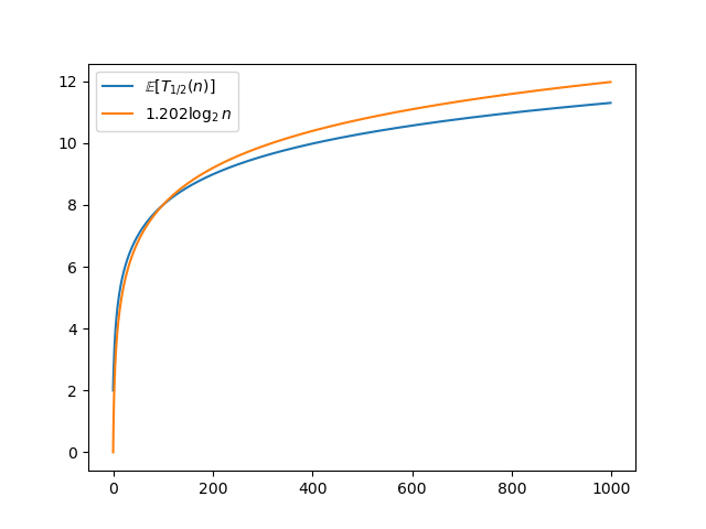
Pretty cool. It seems the result grows rather slowly. In fact, it seems like it grows at the rate of $\bigo{\log n}.$ Here, in this graph, I set the factor so that the graph crosses at $n=100$, so from that point onward, $\ev{T_{1/2}(n)} \leq 1.202 \log_{2} n$.
It’s not enough.
Okay, so, there are a few unsatisfying things about this solution.
For one, you can’t just compute $\evt{n}$ for any $n$ you want. You need to also compute it for all the lower values of $n$. Each computation takes $\bigo{n}$ time so overall you spend $\bigo{n^2}$ time. Can we do better?
Secondly, it just looks scary. Is there an easier solution?
Indeed, there is, but let’s take a step back for the moment. There’s an interesting connection that I want to point out.
Detour: Radioactive decay
In the problem I discussed, the lightbulbs decide whether to turn off or not on each discrete second. In real life, they probably act in a more “continuous” manner. Is there a way we can turn this problem into a continuous version? Indeed, there is!
In the discrete version, the time it takes for a single lightbulb to turn off follows a geometric distribution. The continuous analog of this is called an exponential distribution. Extending this to $n$ lightbulbs is like having $n$ radioactive atoms and then asking about how long we would expect before all atoms finally decay.
Spoiler: The solution is a lot cleaner than the mess we found earlier.
Geometric vs. exponential distribution
Let’s start with just one lightbulb or one atom first.
In the geometric distribution, you can compute the probability that the lightbulb (let’s say, lightbulb numbered $i$) takes exactly $t$ seconds to turn off as
\[\prob{T_{i} = t} = q^{t-1}p,\]or intuitively, the lightbulb fails to turn off for the first $t-1$ seconds with probability $q = 1-p$ each second (independently) then successfully takes the probability $p$ that turns it off at the last second.
Oh, note on notation: $T_i$ is what we call a geometric random variable.
Perhaps, it might be easier to think of this in terms of the cumulative distribution function (CDF), the probability that the lightbulb dies within the first $t$ second:
\[\prob{T_{i} \leq t} = 1-q^{t}.\](Sanity check: $t=0$ means $\prob{T_{i} = 0} = 0$, which makes sense. A lightbulb only ever dies at time $t=1, 2, 3, \cdots$. At $t\to \infty$, the probability approaches 1.)
In the exponential distribution, instead of using the geometric sequence, you use, *drum rolls*, exponential sequence! That is, the exponential random variable $T_i$ has
\[\prob{T_{i} \leq t} = 1 - e^{-\lambda_{i} t},\]where $\lambda_{i}$ is the term that controls the rate of decay; the higher $\lambda_{i}$ is, the more eager the lightbulb is to turn off. We can calculate that $\ev{T_{i}} = \frac{1}{\lambda}$.
Intuitively, an exponential distribution is the limit of geometric progression but with increasingly fine-grained time steps. The probability of success at each time step is very low, but you can set it so that, cumulatively, the probability of success in one second or the expected time to succeed is exactly what you want.
You can’t have both, though! Notice that if you set $\prob{T_{i}\leq1} = 0.5$, then $\lambda_{i} = 0.693$, which means the expected time is $1.443$ seconds. Continuous means there’s more chance for the light to turn off in general, so this is faster than the $2$ seconds we expect in the discrete version.
Similarly, if you want the expected time to be exactly $2$ seconds, then the probability of not finishing within 1 second also has to rise too! The probability of finishing within 1 second falls to $0.393$.
Maximum of exponential variables
Okay, back to the continuous analog of the original problem. We have $n$ lightbulbs. Light bulb $i$ turns off at time $T_i$. $T_1, T_2, \cdots, T_{n}$ are independent and identically distributed (i.i.d.) exponential random variables. What’s the expected time for all light bulbs to be turned off? That is, what is the expected value of $\max \left\{ T_{1}, T_{2}, \cdots, T_{n} \right\}$? This might be familiar to you if you’ve taken the same probability class as I have.
This is tricky, so let’s flip the problem around. If we have $n$ light bulbs, what does the distribution look like for $\min \left\{ T_{1}, T_{2}, \cdots, T_{n} \right\}$? That is, we only care about the time it takes for any light bulb at all to turn off.
The cool thing is, with exponential random variables, the decay rates are additive! If you have $n$ i.i.d. exponential random variables, then their minimum is just an exponential random variable with the summed decay rate.
Therefore, with $n$ light bulbs, the time to wait for any light to turn off is an exponential random variable with $\lambda = n\lambda_{i}$. The expected time is thus simply $\frac{1}{n}$ of one light bulb’s expected time.
We care about the time for all lightbulbs to turn off, though. Leveraging the memoryless property, we can simply add up:
- The time it takes for one of the $n$ lightbulbs to turn off
- The time it takes for one of the remaining $n-1$ lightbulbs to turn off
- The time it takes for one of the remaining $n-2$ lightbulbs to turn off
- and so on… until the time it takes for the final lightbulb to turn off.
Therefore, the formula for $\ev{\widetilde{T_{\lambda}}(n)}$, the expected time for all $n$ lightbulbs to turn off in the continuous version, is
\[\begin{align} \ev{\widetilde{T_{\lambda}}(n)} &= \ev{\widetilde{T_{\lambda}}(1)} \left( 1 + \frac{1}{2} + \frac{1}{3} + \cdots + \frac{1}{n} \right) \\ \\ &= \ev{\widetilde{T_{\lambda}}(1)} \cdot H_{n}, \end{align}\]where $H_n$ is the $n$-th harmonic number. The numbers clearly don’t match our discrete version, regardless of how we tune $\lambda$.
Oh, yeah! Another thing to mention: It is well known that $H_{n}$ is in $\bigo{\log n}$. It grows at roughly the same pace as the discrete version.
A mathematician’s approach
Alright, let’s remember the original problem. We have $n$ lightbulbs. Each might turn off, at each second, with probability $p$. How long does it take for all to turn off, on average?
I asked my mathematician friends to tackle this problem. They don’t have the code-monkey brain-rot symptoms that I do, and sure enough, they found a pretty nice solution.
First, if you’ve done a lot of probability problems, you may be aware of this formula:
\[\evt{n} = \sum_{t=0}^{\infty} \prob{T_{p}(n) > t}.\]Intuitively, we can compute the expected time by adding the probability that we have to take more than 0 seconds, more than 1 second, more than 2 seconds, and so on. In other words, we’re adding the survival function evaluated at each time step. This works because each of them contributes one second, scaled down to whatever probability they happen. Or, if you’d prefer it mathematically, from the definition of expected value:
\[\begin{align} \evt{n} &= \sum_{t=0}^{\infty} \prob{T_{p}(n) = t} \cdot t \\ &= \hphantom{+} \prob{T_{p}(n) = 1} \\ &\,\hphantom{=} + \prob{T_{p}(n) = 2} + \prob{T_{p}(n) = 2} \\ &\,\hphantom{=} + \prob{T_{p}(n) = 3} + \prob{T_{p}(n) = 3} + \prob{T_{p}(n) = 3} \\ &\,\hphantom{=} + \cdots \end{align}\]Sum up the vertical slices to get
\[\evt{n} = \prob{T_{p}(n)>0} + \prob{T_{p}(n)>1} + \prob{T_{p}(n)>2} + \cdots\]Alright. We have to compute $\prob{T_{p}(n) > t}$, the probability that at least one of the lights has failed to turn off in $t$ seconds (so the ultimate time is more than $t$). This is just $1 - \prob{T_{p}(n) \leq t}$: one minus the probability that all lights turn off within the first $t$ seconds.
Whether a lightbulb turns off in the first $t$ seconds or not is completely independent of other lightbulbs, so we can just focus on computing $\prob{T_{p}(1) \leq t}$. This value is simply $1 - q^t$, one minus the probability that the lightbulb fails to turn off $t$ times consecutively.
Overall, we have
\[\begin{align} \evt{n} &= \sum_{t=0}^{\infty} \prob{T_{p}(n) > t} \\ &= \sum_{t=0}^{\infty} \left( 1 - \prob{T_{p}(n) \leq t} \right) \\ &= \sum_{t=0}^{\infty} \left( 1 - \left( \prob{T_{p}(1) \leq t} \right)^n \right) \\ &= \boxed{\sum_{t=0}^{\infty} \left( 1 - \left( 1 - q^t \right)^n \right)}. \end{align}\]We can write this in terms of $p$, our original variable, and get
\[\boxed{\evt{n} = \sum_{t=0}^{\infty} \left( 1 - \left( 1 - \left( 1-p \right) ^t \right)^n \right)}.\]There we go! We’ve got a formula that doesn’t really use any knowledge besides negating probabilities here and there. (Okay, the negations were actually really confusing for me.) No tricky recurrence formula.
B-but… infinite series!
As cool as the new solution is, one issue I have with it is that it is impossible to evaluate exactly as a fraction by hand, due to the infinite sum.
In code, the best we can do is take a finite number of terms ($t$ up to some amount) or take new terms until the answer stops changing by some amount.
import itertools

def close(a, b, epsilon: float = 1e-6):
  if a == 0 or b == 0:
    return a == b
  return abs(a-b)/min(a,b) < epsilon

def infinite_series_solution(N: int, p: float, epsilon: float = 1e-6) -> list[float]:
  q: float = 1-p
  ET: list[float] = [0]*N
  for n in range(N):
    sum: float = 0
    for t in itertools.count():
      diff = 1-(1-q**t)**n
      if close(sum, sum+diff, epsilon):
        break
      sum += diff
    ET[n] = sum
  return ET

if __name__ == "__main__":
  for n, v in enumerate(infinite_series_solution(16, 0.5)):
    print(n,v)
The output is close to what we’ve got from the previous piece of code.
We can do some nasty algebra to get rid of this infinite sum.
First, let’s start here; avoid $p$ because it’s nasty:
\[\evt{n} = \sum_{t=0}^{\infty} \left( 1 - \left( 1 - q ^t \right)^n \right).\]We can expand $\left( 1-q^t \right)^n = \left(-q^t+1 \right)^n$ using binomial expansion.
\[\begin{align} \evt{n} &= \sum_{t=0}^{\infty} \left( 1 - \left( \sum_{k=0}^n \binom{n}{k} (-1)^k q^{kt} \right) \right) \\ &= \sum_{t=0}^{\infty} \left( 1 - \left(1 + \sum_{k=1}^n \binom{n}{k} (-1)^k q^{kt} \right) \right) \\ &= \sum_{t=0}^{\infty} \left( \sum_{k=1}^n \binom{n}{k} (-1)^{k+1} q^{kt} \right) \\ &= \sum_{k=1}^n \left( \binom{n}{k} (-1)^{k+1} \left( \sum_{t=0}^{\infty} q^{kt} \right) \right). \\ \end{align}\]Using the formula for infinite geometric series, we ultimately get
\[\boxed{\evt{n} = \sum_{k=1}^n \left( \binom{n}{k} (-1)^{k+1} \left( \frac{1}{1-q^k} \right) \right)}.\]Again, I confirmed that this solution is correct by coding it up. Got the same solution as earlier!
def binomial_solution(N: int, p: float) -> list[float]:
  q = 1-p
  ET: list[float] = [0]*N
  for n in range(N):
    for k in range(1,n+1):
      ET[n] += C(n,k) * (-1)**(k+1) * 1/(1-q**k)
  return ET

if __name__ == "__main__":
  for n, v in enumerate(binomial_solution(16, 0.5)):
    print(n,v)
Head-to-head comparisons
Alright, for the purpose of this post, let’s say we have found three solutions. I’ll name them:
- The recurrence formula solution
- The infinite series solution
- The binomial solution
Let’s pit them against each other.
Time complexity analysis
As a computer scientist, I am morally obligated to analyze the time and space complexity of all these solutions.
For solution #1, as I’ve mentioned earlier, to compute $\evt{n}$ for arbitrary $n$, you unfortunately have to compute it for all smaller values of $n$ too, so the time complexity required to compute an arbitrary $n$ is $\bigo{n^2}$. The good news is, if you do care about computing it for all $n$ from $0$ up to including or not including $N$, nothing changes, and the time complexity stays at $\bigo{N^2}$.
Actually, while we’re at it, let’s think about space complexity as well. We definitely need $\bigo{n}$ space to store the answers to the subproblems. In the code I provided above, I also spent $\bigo{n^2}$ space on computing $\binom{n}{k}$ but that’s just me being lazy. I used functools.cache, but you could manually write the function bottom-up, store just the last two rows of the Pascal’s Triangle, and it will work just fine. Overall, the space complexity is $\bigo{n}$.
For solution #2, we have a bit of an issue because we are computing with infinite series. If we were to take only a constant number of terms, then given arbitrary $n$, the running time is just $\bigo{1}$. (Obviously, for all $n$ up to $N$, the running time is $\bigo{N}$.) The space complexity is just $O(1)$ for the entire computation as well.
Realistically, we probably want to do something better than just taking a fixed number of terms. We could take a new term if the new term is larger than $\epsilon$, after which we don’t care. That is, we don’t care about $t$ for which
\[\begin{align} 1 - \left( 1 - q^t \right)^n &< \epsilon \\ \left( 1 - q^{t} \right)^{n} &> 1 - \epsilon \\ 1 - q^{t} &> \left( 1 - \epsilon \right)^{1/n} \\ q^{t} &< 1-\left( 1 - \epsilon \right)^{1/n} \\ t &> \log_{q}\left( 1-\left( 1 - \epsilon \right)^{1/n} \right). \end{align}\]We could take new terms as long as the change relative to the current partial sum is large enough (like in my code). We could do a lot of math to figure out exactly how many terms we need to take to ensure the answer is within $\epsilon$ of the true answer, et cetera.
The analyses here are a little bit outside of my expertise, so I’m skipping them. I wouldn’t be surprised if you have to take $\mathrm{\Omega}(n)$ terms for the result to be any good. The value of $q$ might also heavily impact the number of terms as well.
Space complexity is $\bigo{1}$, though. Pretty cool.
For solution #3, given arbitrary $n$, the time complexity is simply $\bigo{n}$. Space complexity is also $\bigo{1}$. It’s not $\bigo{n}$ because turns out it’s also possible to directly compute $\binom{n}{k}$ from $\binom{n}{k-1}$, allowing us to scan across any row in the Pascal’s Triangle without extra space.
As with solution #1, to compute the answers for all $n$ up to $N$, the time complexity is $\bigo{N^2}$. I wonder if we could do better than this at all.
To summarize, solution #2 (infinite series) seems to have the “best” time complexity but that’s probably fake. Solution #3 (binomial) has time complexity of $\bigo{n}$ for arbitrary $n$ and solution #1 (recurrence) has time complexity of $\bigo{n^2}$.
Numerical accuracy
It seems like solution #3 (binomial formula) is the best solution, but that’s actually false!
In the code I provided above, if you try to compute for, say, $n>50$, you’ll find that the answers don’t make sense. At one point, the answers stop being monotonic. At another point, the answers simply cease to follow any pattern at all and just explode to infinity, even at relatively small $n$.
There’s something about the form of this answer that makes it incredibly not suited to floating point computations. I’m not exactly sure what it is exactly, but it could be the alternating positive/negative signs. (I tried many things, though. I summed up the positive and negative parts separately first; I sorted the terms by $\binom{n}{k}$ size and made sure to sum the smaller terms first; etc.)
The other two solutions seem to be fine until $n>1000$, where the values in the computation are either too large ($\binom{n}{k}$) or too small ($q^t$) to fit in a floating point number. I can forgive that.
Overall, solution #1 (recurrence) is better because the formula can be exactly computed. Solution #2 (infinite series) is bound to have some serious floating point errors if you don’t take enough terms.
Actually… how do we know which solution is the one with the “correct” answer?
Computing with fractions
Python is a fun language to use because it comes with so many libraries readily available for explorations like this. Specifically, there is a fractions library that implements rational number arithmetic for us.
We could compute the exact fractions with either solution #1 or #3. Suddenly, all numerical problems with solution #3 disappear! After all, we aren’t dealing with floating point shenanigans.
You can see example results here, for $p=\frac{1}{2}$:
0 0
1 2
2 8/3
3 22/7
4 368/105
5 2470/651
6 7880/1953
7 150266/35433
8 13315424/3011805
9 2350261538/513010785
10 1777792792/376207909
11 340013628538/70008871793
12 203832594062416/40955189998905
13 131294440969788022/25804920098540835
14 822860039794822168/158515937748179415
15 177175812995012739374/33510269239965128331
We could use this method to compute the “ground truth.” We can convert it to a floating point number and compare it to other solution’s answers to see who’s the closest. As discussed earlier, solution #1 indeed gives the closest numerical value.
One important thing to note: Using big integers means you can’t just assume all numerical operations are $\bigo{1}$ anymore, so all the time complexity analyses we did earlier are invalidated. If you want to analyze them properly, you’re welcome to. I’m out.
Summary
| Solution | Time complexity | Space complexity | Numerical accuracy |
|---|---|---|---|
| #1 (Recurrence) | $\bigo{n^2}$ | $\bigo{n}$ | Best |
| #2 (Infinite series) | fake $\bigo{1}$ | $\bigo{1}$ | Acceptable |
| #3 (Binomial formula) | $\bigo{n}$ | $\bigo{1}$ | Simply broken |
OEIS
It turns out we’re not the first to investigate this problem thoroughly. If you take the numerators or the denominators and put them into OEIS, the bible for all the cool integer sequences, you’ll find sequence A158466, titled “Numerators of $\mathrm{EH}(n)$, the expected value of the height of a probabilistic skip list with $n$ elements and $p=1/2$.”
One of the comments states:
$n$ fair coins are flipped in a single toss. Those that show tails are collected and reflipped in another single toss. The process is repeated until all the coins show heads. H(n) is the discrete random variable that denotes the number of tosses required. $\prob{H(n) \leq k} = (1-(1/2)^k)^n$.
This is indeed exactly the same problem! But more interesting, however, are the title and this comment elaborating on the title:
A probabilistic skip list is a data structure for sorted elements with $\bigo{\log n}$ average time complexity for most operations. The probability $p$ is a fixed internal parameter of the skip list.
For some reason, we got ourselves well into computer science territory and stumbled upon skip lists! This post is getting long enough as is, so I’m skipping (pun intended) discussing them.
It seems like no one has found a closed form that’s simpler than any of the solutions we have, though, which is a pity.
Although, I suppose it makes sense. If you look at the harmonic series or the sequence listing A001008, you’ll find that all formulas are large summations, approximations, or ones that rely on other complicated functions (like Stirling numbers of the second kind). So, even for something as “nice” as the harmonic series, there’s really no way to avoid spending a lot of time on computing the $n$-th number.
By the way, some extra connections to make:
- This problem is eerily similar to the coupon collector’s problem.
- The alternating plus/minus sums of the binomial coefficients might remind you of the inclusion-exclusion principle.
- Did you know you could construct the binomial matrix as a very elegant matrix exponential? Absolutely wild.
Alright, I hope you’ve had fun! I’m outta here.